Example I
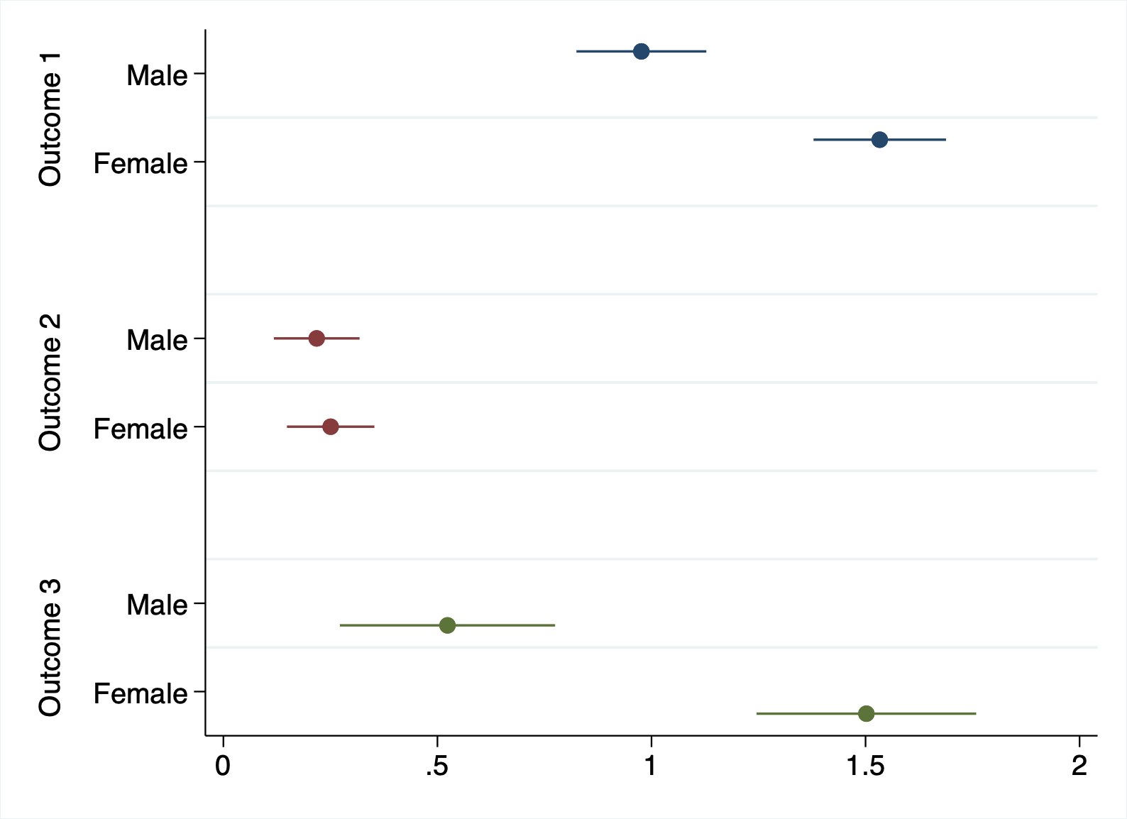
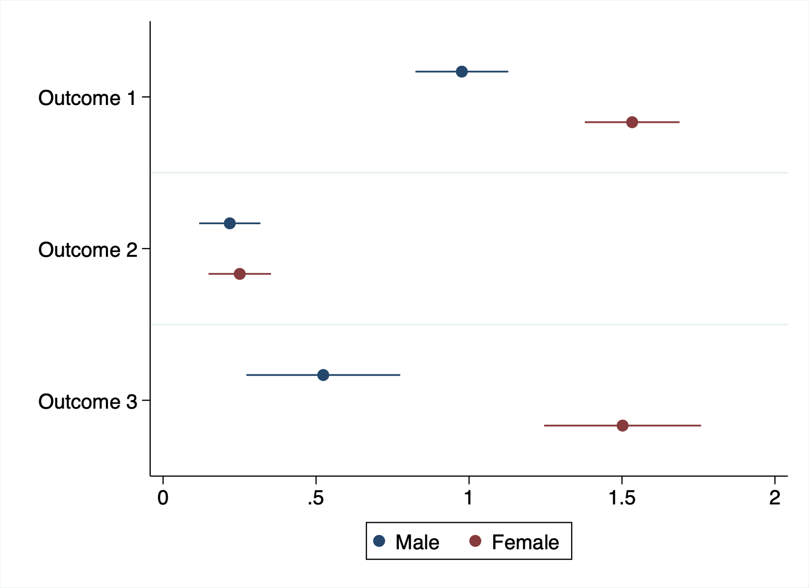
Here you can find two simple examples of plotting results for heterogeneous treatment effects, one by using matrices:
Example


Data set
/*
Let's take some artificial data to show examples of using the coefplot when looking
at heterogeneous treatment effects.
*/

use "example_coefplot.dta", clear


*** First steps: how to test for heterogeneous treatment effects? ***

// Imagine you would like to check for heterogeneous treatment effects on y1
reg 	y1 i.treat##i.female

// What's the total treatment effect for women?
lincom 	1.treat+1.treat#1.female

// Same, but contains total effects for both men and women
contrast r.treat@i.female

// Note that contrast comes with the option "post" to put results in return list


*** Estimate all models & plot them ***

// Loop over all models
local n = 1
foreach outcome in y1 y2 y3 {
	reg `outcome' i.treat##i.female
	contrast r.treat@i.female, post
	est sto e`n'
	local n = `n'+1
}

// Simple coefplot
coefplot e1 e2 e3

// Let's do some refinements: use "aseq" and "eqstrict" to plot results by estimation
coefplot e1 e2 e3, 									///
	aseq eqstrict

// Some cosmetic changes
coefplot e1 e2 e3, 									///
	aseq eqstrict eqlab("Outcome 1" "Outcome 2" "Outcome 3") nokey			///
	coeflab(*0.female="Male" *1.female="Female")					///
	graphr(c(white))


*** More flexible (but also more complicated): Matrices ***

// Create empty matrices
mat A = J(3,3,.)				// matrix to store treatment results for male
mat B = J(3,3,.)				// matrix to store treatment results for female

// Same loop as before, now store results in matrix
local n = 1
foreach outcome in y1 y2 y3 {
	reg `outcome' i.treat##i.female
	mat A[`n',1] = r(table)[1,2]		// coefficient of 1.treat
	mat A[`n',2] = r(table)[5,2]		// lower CI boundary of 1.treat
	mat A[`n',3] = r(table)[6,2]		// upper CI boundary of 1.treat
	lincom 	1.treat+1.treat#1.female
	mat B[`n',1] = r(estimate)		// coefficient of 1.treat+1.treat#1.female
	mat B[`n',2] = r(lb)			// lower CI boundary
	mat B[`n',3] = r(ub)			// upper CI boundary
	local n = `n'+1
}

// Simple coefplot
coefplot (mat(A[.,1]), ci((2 3)))  (mat(B[.,1]), ci((2 3)))

// Some refinements
coefplot (mat(A[.,1]), ci((2 3)))  (mat(B[.,1]), ci((2 3))),  				///
	coeflab(r1="Outcome 1" r2="Outcome 2" r3="Outcome 3") 				///
	plotlab("Male" "Female") graphr(c(white))